Exploring Scottish Peaks

This curated tidytuesday data set comes from The Database of British and Irish Hills. It’s a list of about 600 Scottish mountains that are classified as a Munro, Munro Top, or none. A Munro is a mountain with a distinct summit of and an elevation of at least 3,000 ft (914.4 meters) while a Munro Top is a subsidiary summit on the same mountain that is also over 3,000 feet.

The Database of British and Irish Hills describes a variety of names for peaks of different heights and prominence. For example, peaks that are taller than 2,500 feet and less than 3,000 feet are called Corbetts, while Grahams are between 2,000 and 2,500 feet.

For this example I’ll focus on exploring the data set, cleaning as needed, understanding when mountain peak classifications changed, finding the tallest Munros and Munro tops, and some simple data visualizations.

Code

library(pacman)

p_load(dplyr, tidyr, ggplot2, cowplot, sf, rnaturalearth, ggview)

# scottish munro data is week 33
tuesdata <- tidytuesdayR::tt_load(2025, week = 33)

scot_mun <- tuesdata$scottish_munros

Peeking at Peak Data

Let’s start by learning the data set dimensions and the types of variables in the data set.

Code

# what's in the data set
dplyr::glimpse(scot_mun)

Rows: 604
Columns: 18
$ DoBIH_number <chr> "1", "17", "18", "32", "26", "27", "28", "39", "33", "30"…
$ Name         <chr> "Ben Chonzie", "Ben Vorlich", "Stuc a' Chroin", "Ben Lomo…
$ Height_m     <dbl> 931.0, 985.3, 973.0, 973.7, 1174.0, 1165.0, 1068.0, 923.0…
$ Height_ft    <dbl> 3054, 3233, 3192, 3195, 3852, 3822, 3504, 3028, 3169, 343…
$ xcoord       <dbl> 277324, 262912, 261746, 236707, 243276, 243481, 243842, 2…
$ ycoord       <dbl> 730857, 718916, 717465, 702863, 724417, 722712, 722052, 7…
$ `1891`       <chr> "Munro", "Munro", "Munro", "Munro", "Munro", "Munro", "Mu…
$ `1921`       <chr> "Munro", "Munro", "Munro", "Munro", "Munro", "Munro", "Mu…
$ `1933`       <chr> "Munro", "Munro", "Munro", "Munro", "Munro", "Munro", "Mu…
$ `1953`       <chr> "Munro", "Munro", "Munro", "Munro", "Munro", "Munro", "Mu…
$ `1969`       <chr> "Munro", "Munro", "Munro", "Munro", "Munro", "Munro", "Mu…
$ `1974`       <chr> "Munro", "Munro", "Munro", "Munro", "Munro", "Munro", "Mu…
$ `1981`       <chr> "Munro", "Munro", "Munro", "Munro", "Munro", "Munro", "Mu…
$ `1984`       <chr> "Munro", "Munro", "Munro", "Munro", "Munro", "Munro", "Mu…
$ `1990`       <chr> "Munro", "Munro", "Munro", "Munro", "Munro", "Munro", "Mu…
$ `1997`       <chr> "Munro", "Munro", "Munro", "Munro", "Munro", "Munro", "Mu…
$ `2021`       <chr> "Munro", "Munro", "Munro", "Munro", "Munro", "Munro", "Mu…
$ Comments     <chr> NA, NA, NA, NA, NA, "1891: Am Binnein (Stobinain)", NA, N…

Code

# how many missing values in the year columns?
# sapply(scot_mun[,7:17], function(x) sum(is.na(x)))

We can use the DT package to more closely examine the comments and geographical classification as of 2021.

Code

# include the most recent year only.

scot_mun |> 
  select(DoBIH_number, Name, Height_ft,
         `2021`, Comments) |> 
  DT::datatable(colnames = c("DoBIH #", "Name", "Height (ft)", "Category 2021", "Comments"),
                rownames = FALSE,
                options = list(pageLength = 5, language = list(search = 'Filter:'),
                               lengthMenu = c(5, 10, 25, 50))
                )

We can see some additional cleaning is needed as the last entry in the dataset is a comment rather than a peak. This explains why DoBIH_number is coded as a character variable rather than as an integer.

From the comments we can see that a number peaks have been reclassified over the years. For example, the peak Beinn a’ Chlaidheimh was classified as a Munro in 1974, but after a geological survey in 2011 found that it was in fact just shy of the 3,000 ft cutoff to be labelled a Munro! Today Beinn a’ Chlaidheimh is classified as a Corbett. This would explain by peaks with an elevation of less than 3,000 ft don’t have a category listed, but others are tall enough to meet the threshold for Munros but lack a label.

For example, why doesn’t the peak Stob Binnein - Creag a’ Bhragit (DoBIH #39) with a height of 3,082 ft have a designated category? No explanation is given in the comments column, but the Database of British and Irish Hills website states that remapping efforts have resulted in many Monro Tops being deleted on subjective grounds. Some further digging in the Database’s changelog confirms that this peak is a deleted Munro Top.

Code

scot_mun |> 
  filter(Name %in% c("Beinn a' Chlaidheimh")) |> 
  tidyr::pivot_longer(cols = 7:17, names_to = "year", values_to = "class") |> 
  mutate(year = as.integer(year)) |> 
  arrange(DoBIH_number, Name, year) |>
  select(year, class) |> 
  knitr::kable(col.names = c("Year", "Classification"),
               caption = "Classification over time for Beinn a' Chlaidheimh")

Classification over time for Beinn a’ Chlaidheimh
Year	Classification
1891	NA
1921	NA
1933	NA
1953	NA
1969	NA
1974	Munro
1981	Munro
1984	Munro
1990	Munro
1997	Munro
2021	NA

Let’s finish with a final examination of peak classification over time.

Code

scot_long <- scot_mun[-604,] |> 
  tidyr::pivot_longer(cols = 7:17, names_to = "year", values_to = "class") |> 
  mutate(year = as.integer(year)) |> 
  arrange(DoBIH_number, Name, year)

scot_long |> 
    mutate(class = tidyr::replace_na(class, "none listed")) |> 
  group_by(year, class) |> 
  summarise(n = n()) |> 
  pivot_wider(names_from = class, values_from = n) |> 
  knitr::kable(col.names = c("Year", "Munro", "Munro Top", "Other"),
               caption = "Peak categories over the years.")

Peak categories over the years.
Year	Munro	Munro Top	Other
1891	283	255	65
1921	276	267	60
1933	276	267	60
1953	276	267	60
1969	276	267	60
1974	279	262	62
1981	276	241	86
1984	277	240	86
1990	277	240	86
1997	284	227	92
2021	282	226	95

Code

# add column that designates a classification switch
scot_long <- scot_long |> 
  group_by(DoBIH_number) |> 
  mutate(class_lag = lag(class),
         switch = case_when(class == class_lag ~ NA,
                            class != class_lag ~ "switch")) |> 
  select(-class_lag)

# which year saw the greatest number of 
# classification switches?
scot_long |> 
  mutate(switch = replace_na(switch, "no switch")) |> 
  group_by(year, switch) |> 
  summarise(n = n()) |> 
  pivot_wider(names_from = switch, values_from = n) |> 
  mutate(switch = replace_na(switch, 0)) |> 
  dplyr::select(-`no switch`) |> 
  knitr::kable(col.names = c("Year", "n"),
              caption = "Number of Category Switches Each Year") |> 
  kableExtra::kable_styling(bootstrap_options = "striped", full_width = F)

Number of Category Switches Each Year
Year	n
1891	0
1921	33
1933	2
1953	0
1969	0
1974	3
1981	16
1984	0
1990	0
1997	10
2021	1

Code

# was any peak re-designated more than once?
scot_long |> 
  dplyr::filter(switch == "switch") |> 
  group_by(DoBIH_number, Name) |> 
  summarise(n = n()) |> 
  dplyr::filter(n > 1) |> 
  arrange(Name)

switch_ids <- as.character(c(312, 315, 809, 523, 308, 1010))

A small handful of peaks were re-classified more than once. The table below lists what these peaks were originally classified as and the years it was changed.

Code

switch_tab <- scot_long |> 
  dplyr::filter(DoBIH_number %in% switch_ids) |> 
  select(DoBIH_number, Name, year, switch, class) |>
  dplyr::filter(switch == "switch") |> 
  dplyr::select(-switch) |> 
  arrange(Name, year)


pre_switch <- scot_long |> 
  dplyr::filter(DoBIH_number %in% switch_ids) |> 
  #dplyr::filter(!is.na(class)) |> 
  select(DoBIH_number, Name, year, class, switch) |> 
  group_by(DoBIH_number) |> 
  mutate(test = lead(switch, n = 1),
         pre_switch = case_when(is.na(switch) & test == "switch" ~ "pre")) |> 
  select(-test) |> 
  dplyr::filter(pre_switch == "pre") |> 
  slice_head(n = 1) |> 
  select(-switch, -pre_switch)

switch_table <- rbind(switch_tab, pre_switch)

switch_table |> 
  arrange(Name, year) |> 
  knitr::kable(col.names = c("DoBIH #", "Name", "Year", "Class"),
               caption = "Mountains re-classified more than once.") |> 
  kableExtra::kable_paper(full_width = F) |> 
  kableExtra::row_spec(c(1:3, 7:9, 13:15), background = "#D9D9D9")

Mountains re-classified more than once.
DoBIH #	Name	Year	Class
312	An Gearanach	1891	Munro
312	An Gearanach	1921	Munro Top
312	An Gearanach	1933	Munro
315	An Gearanach - An Garbhanach	1891	Munro Top
315	An Gearanach - An Garbhanach	1921	Munro
315	An Gearanach - An Garbhanach	1933	Munro Top
523	Sgor an Lochain Uaine	1891	Munro
523	Sgor an Lochain Uaine	1921	Munro Top
523	Sgor an Lochain Uaine	1997	Munro
308	Sgurr a' Mhaim - Sgurr an Iubhair [Sgor an Iubhair]	1974	Munro Top
308	Sgurr a' Mhaim - Sgurr an Iubhair [Sgor an Iubhair]	1981	Munro
308	Sgurr a' Mhaim - Sgurr an Iubhair [Sgor an Iubhair]	1997	Munro Top
1010	Slioch	1974	Munro
1010	Slioch	1981	Munro Top
1010	Slioch	1997	Munro

A bit of cleaning & processing

The data needs to be prepared further before I can proceed with a simple statistical summary and visuals. I’m going to remove the entry that’s actually a comment as well as all entries that are not Munros or Munro Tops in 2021.

Code

scot_mun_clean <- scot_mun[-604,] |> 
  dplyr::filter(!is.na(`2021`))

Elevation Statistics

Code

scot_mun_clean |> 
  group_by(`2021`) |>
  summarise(n = n(),
            smallest = min(Height_ft),
            tallest = max(Height_ft),
            average = mean(Height_ft),
            median = median(Height_ft)) |> 
  knitr::kable(digits = 0,
               col.names = c("", "n", "Shortest", "Tallest", "Average", "Median"),
               caption = "Peak Summary Statistics")

Peak Summary Statistics
	n	Shortest	Tallest	Average	Median
Munro	282	3001	4411	3339	3277
Munro Top	226	3001	4150	3269	3198

Code

scot_mun_clean |> 
  select(DoBIH_number, Name, Height_ft, `2021`) |> 
  group_by(`2021`) |> 
  dplyr::arrange(desc(Height_ft)) |> 
  slice_head(n = 10) |> 
  ungroup() |> 
  mutate(Name = forcats::fct_reorder(Name, Height_ft)) %>%
  ggplot(aes(x = Name,
             y = Height_ft)) +
  # set geom lower limit to 3000 b/c munros are at least 3001
  geom_segment(aes(xend = Name, yend = 3000)) +
  geom_point(aes(color = `2021`, shape = `2021`),
             size = 4) +
  labs(y = "Height (ft)",
       x = "",
       title = "Ten Tallest Munros & Munro Tops") +
  theme_classic() +
  theme(plot.title = element_text(hjust = -1),
        legend.position = "bottom",
        legend.title = element_blank()) +
  scale_color_manual(values = c("#117A8B", "#79115C")) +
  scale_shape_manual(values = c(15, 19)) +
  coord_flip()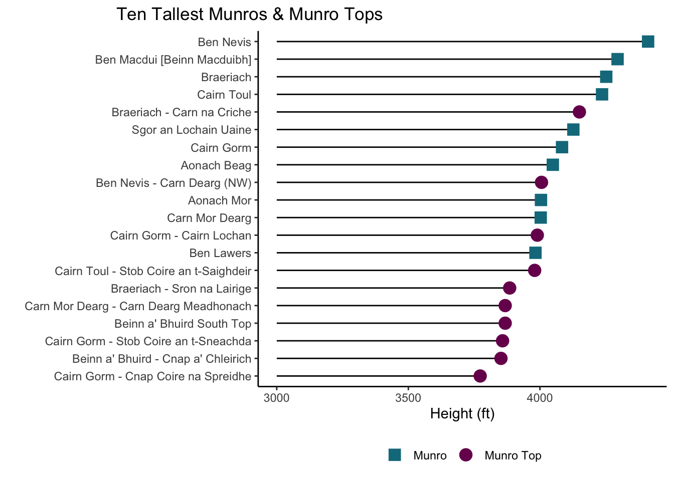

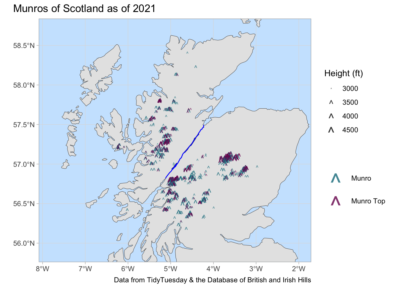
Mapping the peaks

The coordinates given use the British National Grid (OSGB36) projection. I want to transformed these coordinates to EPSG 4326 (used for GPS).

Code

# some geographic info
# fetch county shape for Scotland
scotland <- rnaturalearth::ne_countries(geounit = "scotland", 
                                        type = "map_units",
                                        scale="large")

# fetch spatial information for water features
water <-rnaturalearth:: ne_download(scale=10, 
                                    type="lakes", 
                                    category="physical")

# fetch spatial information for rivers
river <- ne_download(scale=10, 
                     type="rivers_lake_centerlines", 
                     category="physical")

sf_use_s2(FALSE)
waterscotland <- st_filter(water, scotland)
riverscotland <- st_filter(river, scotland)

munros2021 <- scot_mun_clean |> 
  select(DoBIH_number, Name, Height_m, Height_ft, xcoord, ycoord, `2021`, Comments) |> 
  dplyr::filter(`2021` %in% c("Munro", "Munro Top"))


# crs EPSG 27700 = British National Grid -- United Kingdom Ordnance Survey
# crds EPSG 4326 = World Geodetic System 1984, used in GPS
projection <- st_as_sf(scot_mun_clean |> 
                         filter(!is.na(xcoord),
                                !is.na(ycoord)),
                       coords=c("xcoord","ycoord"),
                       crs = 27700) |> 
  st_transform(crs=4326) |> 
  st_coordinates()

scot_mun_clean <- scot_mun_clean |> 
  filter(!is.na(xcoord)) |> 
  cbind(projection)

Code

# reminder: X is longitude, Y is latitude

scotland |> 
  ggplot() +
  geom_sf() +
  geom_sf(data=waterscotland, fill="blue") +
  geom_sf(data=riverscotland, color="blue") +
  geom_point(data=scot_mun_clean, 
             aes(x=X, 
                 y=Y, 
                 color=`2021`, 
                 size = Height_ft),
             shape="^",
             alpha = 0.8) +
  theme_light() +
  coord_sf(xlim=c(-7.8,-2), 
           ylim = c(55.9, 58.7)) +
  scale_color_manual(values = c("#117A8B", "#79115C")) +
  scale_size_continuous(limits=c(3000, 4500), 
                         breaks=seq(3000, 45000, by=500)) +
  labs(color="",
       title="Munros of Scotland as of 2021",
       caption="Data from TidyTuesday & the Database of British and Irish Hills") +
  theme(legend.position="right",
        plot.title.position="plot",
        axis.title = element_blank(),
        panel.background = element_rect(fill="#cce6fe"),
        legend.key = element_rect(fill = NA)) +
  guides(color = guide_legend(override.aes = list(size = 10)),
         size = guide_legend(title = "Height (ft)"))