Earthquake Frequency, Fear, and Preparedness

It’s actually quite terrifying that the ground can unexpectedly, violently spasm

On August 23, 2011, a 5.8 magnitude earthquake struck Virginia and memes poking fun at alarmed reactions soon followed.

I suspect these memes were most enjoyed by those living in more earthquake prone areas, but earthquakes are relatively rare in the Eastern side of US compared to the Western states. In 2025, there were only 2 recorded quakes with a magnitude greater than 2.5 within the state of Virginia. Within all of the states on the Eastern Seaboard, only 16 quakes of 2.5+ magnitude were recorded with the largest having a magnitude of 3.26. In comparison, 679 earthquakes of magnitude 2.5 or greater were recorded in California last year.

This 2011 Virginia quake was felt by millions and was very likely many people’s very first earthquake experience. Thus, it’s like that the fear of and preparedness for earthquakes is relative to people’s geographic location as well as prior experience.

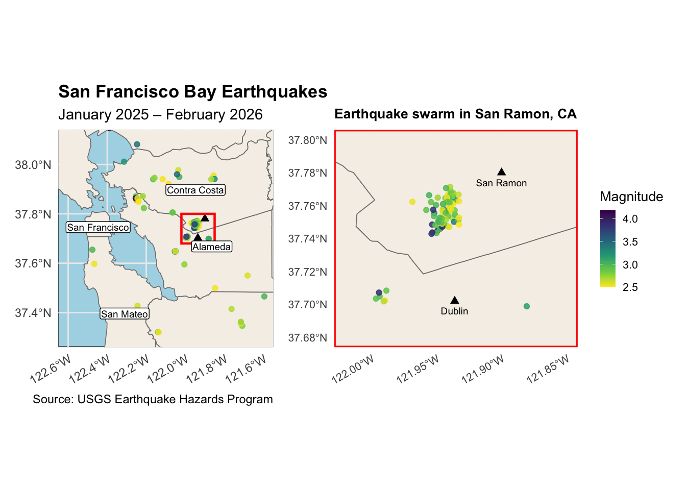
In this post, I’m going to explore 2025 USA earthquake data sourced from the USGS with an initial focus on a cluster of tremors in a neighborhood of San Ramon, CA followed by a wider examination of occurences across the nation. Additionally, the fivethirtyeight package has a data set called san_andreas which is a collection of survey responses that asked people about their fear of quakes, the “Big One”, US region, and prior experience. The data set is named after a 2015 movie named “San Andreas” which is about the aftermath of a massive earthquake caused by the San Andreas Fault. Colloquially, the “Big One” refers to the anticipation of the next big >7.0 quake along this fault line.

Here’s a basic outline of what I’ll go over:

1. San Ramon Earthquake Swam
   1. Explore number and magnitude of quakes recorded between Jan 1, 2025 and Feb 10, 2026
   2. Data visualizations of the swarm
2. Earthquake Frequency by US Region
   1. Explore and prepare the USGS data
   2. Interactive map showing quake frequency by state
   3. Maps comparing Mountain region and parts of the East Coast near Virginia
   4. Table of quakes by region and state
3. fivethirtyeight data describing fear of quakes by region
   1. Examine preparedness by prior experience and region
   2. Examine general fear of quakes by region
   3. Link to Shiny app

library(pacman)

p_load(dplyr, ggplot2, tidyr, sf, spData, tigris, gganimate, av, ggspatial, patchwork, plotly, gt, usmap)
# cache downloads so you're not re-downloading every session
options(tigris_use_cache = TRUE)

# get quake worry data from 538 package
san_andreas <- fivethirtyeight::san_andreas

usa_quakes <- readr::read_csv("all_quakes2025.csv")

# quakes in san ramon from 1/1/25 to 2/11/26
sr_quakes <- readr::read_csv("sanramon.csv")
# and quakes all around the sf bay area
bayarea <- readr::read_csv("bayarea_quakes.csv")

# havent' updated dplyr yet for filter_out
`%notin%` <- Negate(`%in%`)

Earthquake Swarm in San Ramon

# Convert to an sf object
# This adds a geometry column from your lat/lon columns
# this is san ramon specific -- the smaller inset map
sanramon_sf <- st_as_sf(
  sr_quakes,
  coords = c("longitude", "latitude"),  # x first, then y
  crs = 4326,
  remove = FALSE  # keep the original lat/lon columns too
)

# for the wider bay area -- the larger map
bayarea_sf <- st_as_sf(
  bayarea,
  coords = c("longitude", "latitude"),  # x first, then y
  crs = 4326,
  remove = FALSE  # keep the original lat/lon columns too
)


# Download California county boundaries
ca_counties <- tigris::counties(state = "CA", cb = TRUE) |> 
  sf::st_transform(4326)  # make sure CRS matches our earthquake data

# Using a single object means the rectangle and the inset zoom
# are guaranteed to match each other — no copy-paste errors
# smaller inset
inset_xlim <- c(-122.02, -121.85)
inset_ylim <- c(37.68, 37.8)

# add a couple of city landmarks
landmarks <- data.frame(
  name = c("San Ramon", "Dublin"),
  lon  = c(-121.900, -121.936),
  lat  = c(37.780,   37.702)
  )

# Map 1: Bay Area overview ---
map_overview <- ggplot() +
  geom_sf(data = ca_counties,
          fill = "#f5f0e8",
          color = "gray50",
          linewidth = 0.3) +
  geom_sf(data = sanramon_sf,
          aes(color = mag),
          alpha = 0.85
          ) +
  geom_sf(data = bayarea_sf,
          aes(color = mag),
          alpha = 0.85
          ) +
  geom_point(data = landmarks,
             aes(x = lon, y = lat),
             shape = 17,      # filled triangle shape
             size = 2,
             color = "black"
             ) +
  scale_color_viridis_c(
    name = "Magnitude",
    option = "viridis",
    direction = -1 # reverse direction for color gradient intution
    ) +
  # Draw the rectangle using the same coords as the inset
  # This is what visually connects the two maps
  # put the rectangle UNDER geom_sf_labels, else it might cover a label
  geom_rect(
    aes(xmin = inset_xlim[1], xmax = inset_xlim[2],
        ymin = inset_ylim[1], ymax = inset_ylim[2]),
    fill = NA,         # transparent interior
    color = "red",     # red border so it stands out
    linewidth = 0.8
    ) +
  geom_sf_label(data = ca_counties,
                aes(label = NAME),
                size = 2.5,
                nudge_y = -0.012,
                label.padding = unit(0.1, "lines")) +
  coord_sf(xlim = c(-122.6, -121.6), ylim = c(37.3, 38.1)) +
  labs(
    title = "San Francisco Bay Earthquakes",
    subtitle = "January 2025 – February 2026",
    caption = "Source: USGS Earthquake Hazards Program",
    x = NULL, y = NULL
  ) +
  theme_minimal() +
  theme(
    plot.title = element_text(face = "bold", size = 13),
    axis.text.x = element_text(angle = 30, hjust = 1),
    panel.background = element_rect(fill = "lightblue"),
    # remove legend from overview — it lives in the inset
    legend.position = "right"  
  )

# Map 2: San Ramon detail inset ---
map_inset <- ggplot() +
  geom_sf(data = ca_counties,
          fill = "#f5f0e8",
          color = "gray50",
          linewidth = 0.3) +
  geom_sf(data = sanramon_sf,
          aes(color = mag),  
          alpha = 0.85
  ) +
  scale_color_viridis_c(
    name = "Magnitude",
    option = "viridis",
    direction = -1
  ) +
  coord_sf(xlim = inset_xlim, 
           ylim = inset_ylim) +
  labs(
    title ="Earthquake swarm in San Ramon, CA",
    x = NULL, 
    y = NULL
  ) +
  theme_minimal() +
  theme(
    plot.title = element_text(size = 8, face = "bold"),
    plot.caption = element_text(size = 6),
    axis.text = element_text(size = 6),
    axis.text.x = element_text(angle = 30),
    legend.position = "none",
    legend.title = element_text(size = 7),
    legend.text = element_text(size = 6),
    legend.key.size = unit(0.4, "cm"),
    plot.background = element_rect(fill = "#f5f0e8",
                                   color = "red", 
                                   linewidth = 0.8)
  ) + 
  geom_point(data = landmarks,
           aes(x = lon, y = lat),
           shape = 17,      
           size = 2,
           color = "black") +
  geom_text(data = landmarks,
            aes(x = lon, y = lat, label = name),
            size = 2.5,
            nudge_y = -0.006)  # shift label slightly below the point

# Embed the inset into the overview ---
# annotation_custom() places a grob at specific coordinates
# grob is the smaller map inset of san ramon
# The x/y values here are in the DATA coordinates of map_overview
# so we use longitude/latitude values to position it
map_final <- map_overview +
  annotation_custom(
    grob = ggplotGrob(map_inset),  # convert ggplot to embeddable grob
    xmin = -122.13, xmax = -121.55, # horizontal position in lon degrees
    ymin = 37.28,   ymax = 37.62   # vertical position in lat degrees
  ) +
  # add line segments to connect the small red rectangle to map inset
  annotate("segment",
           x = -122.02,
           xend = -122.065,
           y = 37.68, 
           yend = 37.62,
           color = "red",
           linewidth = 0.8) +
  annotate("segment",
           x = -121.85,
           xend = -121.61,
           y = 37.68, 
           yend = 37.62,
           color = "red",
           linewidth = 0.8)

#map_final

# show this visual instead.
# I like the map inset version but it doesn't resize
# when rendered on blog


# alter the inset map to be an adjacent map
# red border interior instead of exterior
# resize labels
# add legend

map_inset2 <- ggplot() +
  geom_sf(data = ca_counties,
          fill = "#f5f0e8",
          color = "gray50",
          linewidth = 0.3) +
  geom_sf(data = sanramon_sf,
          aes(color = mag),  
          alpha = 0.85
  ) +
  scale_color_viridis_c(
    name = "Magnitude",
    option = "viridis",
    direction = -1
  ) +
  coord_sf(xlim = inset_xlim, 
           ylim = inset_ylim) +
  labs(
    subtitle ="Earthquake swarm in San Ramon, CA",
    x = NULL, 
    y = NULL
  ) +
  theme_minimal() +
  theme(
    plot.subtitle = element_text(size = 10, face = "bold"),
    plot.caption = element_text(size = 6),
    axis.text = element_text(size = 8),
    axis.text.x = element_text(angle = 30, hjust = 1),
    legend.position = "right",
    legend.title = element_text(size = 10),
    legend.text = element_text(size = 8),
    legend.key.size = unit(0.4, "cm"),
    panel.border = element_rect(fill = NA,
                                color ="red",
                                linewidth = 1),
    panel.background = element_rect(fill = "#f5f0e8"),
  ) + 
  geom_point(data = landmarks,
           aes(x = lon, y = lat),
           shape = 17,      
           size = 2,
           color = "black") +
  geom_text(data = landmarks,
            aes(x = lon, y = lat, label = name),
            size = 2.5,
            nudge_y = -0.006)



map_overview2 <- map_overview + theme(legend.position = "none")
map_overview2 + map_inset2

Earthquakes are very common in California, and a series of small, localized earthquakes over a relatively short period of time is called an earthquake swarm. One neighborhood in San Ramon has experienced a very high number of number of tremors. According to USGS, there have been 83 recorded earthquakes (with magnitude <= 2.5) over 29 days between 2025 and the first few months of this year. On February 2, 2026, alone there were 22 earthquakes of magnitude 2.5 or greater.

# glimpse(sr_quakes)

# lubridate::date(sr_quakes$time) |> head()

# add date column to san ramon quakes
sr_quakes$date <- lubridate::date(sr_quakes$time)
sr_quakes <- sr_quakes |> relocate(date, .after = time)
#length(unique(sr_quakes$date)) # 29 days of quakes over this time period
#nrow(sr_quakes) # 83 quakes total


# number of quakes by day in san ramon
table(sr_quakes$date)

2025-03-18 2025-03-22 2025-04-01 2025-05-16 2025-07-01 2025-09-07 2025-11-09 
         2          2          1          1          1          1          7 
2025-11-10 2025-11-18 2025-11-20 2025-12-08 2025-12-13 2025-12-15 2025-12-16 
         1          2          1          8          1          1          1 
2025-12-17 2025-12-20 2025-12-21 2025-12-23 2025-12-24 2025-12-28 2026-01-02 
         1          5          3          1          1          2          1 
2026-01-09 2026-01-11 2026-01-30 2026-02-02 2026-02-03 2026-02-05 2026-02-06 
         3          2          3         22          5          2          1 
2026-02-10 
         1 

# largest and smallest quake on feb 2, 2026
sr_quakes |> 
  dplyr::filter(date == "2026-02-02") |> 
  summarise(number = n(),
            "Smallest Magnitude" = min(mag),
            "Largest Magnitude" = max(mag)) |> 
  knitr::kable(caption = "Earthquake Swarm in San Ramon, CA on Feb 2, 2026")

Earthquake Swarm in San Ramon, CA on Feb 2, 2026

number	Smallest Magnitude	Largest Magnitude
22	2.5	4.18

# show the code but do not execute

# add shape file info for quake coordinates
points_sf <- st_as_sf(sr_quakes,
                      coords = c("longitude", "latitude"), 
                      crs = 4326)

sr_quake_plot2 <- ggplot() +
  ggspatial::annotation_map_tile() +
  geom_sf(data = points_sf,
          aes(size = mag,
              color = mag,
              group = seq_along(date))
  ) +
  coord_sf(expand = FALSE) +
  scale_color_viridis_c(guide = "legend",
                        option = "C",
                        direction = -1) +
  scale_size_continuous(range = c(1, 6)) +
  # combine the legends into a single legend
  guides(color = guide_legend(title = "magnitude"),
         size = guide_legend(title = "magnitude")) +
  # transition between several distinct stages of the data
  gganimate::transition_states(date, 
                               transition_length = 3, 
                               state_length = 1) +
  # use these animates b/c quakes are distinct data points
  gganimate::enter_grow() +
  gganimate::exit_shrink() +
  labs(title = "Date: {closest_state}")

# for making mp4 videos
animated_quake_plot2 <- animate(sr_quake_plot2, 
                               nframes = 150,
                               fps = 5,
                               renderer = av_renderer())
animated_quake_plot2
gganimate::anim_save(filename = "animated_quake_plot2.mp4")

Earthquake Frequency by US Region

Preparing and exploring 2025 USA Quake Data

As with the Bay Area earthquake data, these data resourced from the USGS. I had to download a few different files to get information for the conterminous US, Hawaii, and Alaska. Interestingly, these downloads included quakes with coordinates in Canada and Mexico. While tremors can be felt across boarders, I decided to filter them out of this analysis as I want to examine this data in context of the san_andreas survey responses. Only quakes with coordinates that fall within a states boundaries or just off-shore will be included.

Understanding how frequently earthquakes strike in different US regions may help us understand respondents fear and preparedness in the fivethirtyeight survey.

Some notes on USGS data preparation

• The minimum magnitude in this data set is 2.5. While earthquakes of smaller magnitudes are detectable, I decided to limit my focus to quakes that most people can perceive. Generally speaking, most people don’t notice a quake that is smaller than 2.5.

• Continental USA data was joined with data sets collected from manually selected boxed boundaries around Alaska and Hawaii. These boundaries were arbitrary on my part.

• This data set includes off-shore earthquakes as well as a few in Canada and Mexico.

• Columns for state name, US census region, and country (USA, Canada, and Mexico) will be manually added.

• The USGS includes columns for the epicenter’s latitude and longitude as well as a column called place. place is the nearest named geographic region to the earthquake , and it’s useful for confirming the correct state and country has been assigned.

Let’s start with examining the content of the usa_quakes data downloaded from the USGS website and add additional geographical information with the aid of the sf and tigris packages.

# head(usa_quakes) |> glimpse()


# add geographical information ----

# add geographical information to usa_quakes
# shape files, nearest USA state
# this code should add a geometry column
# the geometry type added is POINT
usa_quakes <- st_as_sf(
  usa_quakes,
  coords = c("longitude", "latitude"),
  # crs 4326 = WGS 84 -- very widely used ref system
  crs = 4326, 
  remove = FALSE
)

#head(usa_quakes) |> glimpse() # geometry column added to df

## get state and territory map shape info ----
# load USA polygons
# download shapefile for all states
states_sf <- tigris::states(cb = TRUE) %>%
  sf::st_transform(4326) %>% # transform or covert coordinates of simple feature
  select(state = NAME)

# note the geometry column, includes territories
# the geometry column is a multipolygon, this should be the outline of the state or territory
# territories will not be included in following analyses
#head(states_sf)

## spatial join and drop geometry ----
# st_join == spatial join
# st_within == geometric binary predicates on pairs of simple geometry sets
usa_quakes <- sf::st_join(usa_quakes, states_sf, join = st_within)

head(usa_quakes) |> glimpse() # joined on geo column, new state column added

Rows: 6
Columns: 24
$ time            <dttm> 2025-12-31 23:24:31, 2025-12-31 20:44:09, 2025-12-31 …
$ latitude        <dbl> 40.48983, 44.66417, 32.30740, 38.83150, 40.53300, 40.5…
$ longitude       <dbl> -124.7932, -110.6783, -104.4981, -122.8120, -120.6768,…
$ depth           <dbl> 22.310, 7.400, 5.495, 2.010, 6.430, 5.320
$ mag             <dbl> 2.74, 2.71, 2.70, 2.88, 2.50, 4.92
$ magType         <chr> "md", "ml", "ml", "md", "md", "mw"
$ nst             <dbl> 67, 27, 29, 108, 25, 29
$ gap             <dbl> 236, 43, 88, 21, 61, 62
$ dmin            <dbl> 0.338700, 0.048630, 0.526000, 0.008232, 0.095200, 0.08…
$ rms             <dbl> 0.16, 0.18, 0.20, 0.08, 0.13, 0.16
$ net             <chr> "nc", "uu", "us", "nc", "nc", "nc"
$ id              <chr> "nc75289406", "uu80126531", "us7000rlr4", "nc75289026"…
$ updated         <dttm> 2026-01-27 04:37:24, 2026-01-14 17:57:11, 2026-01-22 1…
$ place           <chr> "46 km WSW of Ferndale, CA", "33 km E of West Yellowst…
$ type            <chr> "earthquake", "earthquake", "earthquake", "earthquake"…
$ horizontalError <dbl> 0.77, 0.28, 2.31, 0.08, 0.21, 0.23
$ depthError      <dbl> 1.760, 0.450, 5.746, 0.130, 0.590, 0.840
$ magError        <dbl> 0.316000, 0.305699, 0.060000, 0.172000, 0.162000, NA
$ magNst          <dbl> 44, 11, 70, 150, 30, 20
$ status          <chr> "reviewed", "reviewed", "reviewed", "reviewed", "revie…
$ locationSource  <chr> "nc", "uu", "us", "nc", "nc", "nc"
$ magSource       <chr> "nc", "uu", "us", "nc", "nc", "nc"
$ geometry        <POINT [°]> POINT (-124.7932 40.48983), POINT (-110.6783 44.66417)…
$ state           <chr> NA, "Wyoming", "New Mexico", "California", "California…

# relocate state to after place column
usa_quakes <- usa_quakes |> 
  relocate(state, .after = place)

There are 9,207 observations in the usa_quakes data set. After the state geometry information we see that 37 states are represented, but state information is missing for 5,931 rows. This is because off-shore or quakes outside of the country will have longitude and latitude coordinates fall outside of state boundary.

# data assessment prior to mapping ----
# additional cleaning and wrangling may be required

## add missing state information ----
# check for missing info and states with earthquakes recorded
sum(is.na(usa_quakes$state)) # 5931 rows without states

[1] 5931

length(unique(usa_quakes$state)) # 37 states represented

[1] 37

table(usa_quakes$state)

        Alaska        Arizona       Arkansas     California       Colorado 
          1162             24              3            679              7 
       Georgia         Hawaii          Idaho       Illinois        Indiana 
             1            139            125              2              1 
        Kansas       Kentucky      Louisiana          Maine       Maryland 
            65              2              5              1              1 
   Mississippi       Missouri        Montana       Nebraska         Nevada 
             1             10             29              3            279 
    New Jersey     New Mexico       New York North Carolina           Ohio 
             2             74              2              1              7 
      Oklahoma         Oregon   Pennsylvania South Carolina   South Dakota 
            29              6              1              5              3 
     Tennessee          Texas           Utah       Virginia     Washington 
             7            488             19              2             47 
       Wyoming 
            44 

A small sample of rows without a state show some earthquakes that struck off the coast of California or have coordinates in Canada or Mexico.

# let's look at some rows without states
# some quakes are near california islands
# others are off the coast of british columbia or Mexico's baja ca
usa_quakes |> 
  dplyr::filter(is.na(state)) |> 
  select(place, state) |> 
  head(10) |> 
  sf::st_drop_geometry() |> 
  knitr::kable(caption = "Sample of eqicenters outside of US State borders")

Sample of eqicenters outside of US State borders

place	state
46 km WSW of Ferndale, CA	NA
46 km W of Puerto Peñasco, Mexico	NA
39 km WNW of Petrolia, CA	NA
54 km W of Petrolia, CA	NA
15 km S of Santa Rosa Is., CA	NA
9 km S of Carpinteria, CA	NA
36 km WNW of Petrolia, CA	NA
10 km WSW of Malibu, CA	NA
90 km SSW of Alberto Oviedo Mota, B.C., MX	NA
14 km N of Saint-Pascal, Canada	NA

missing10_sample <- usa_quakes |> 
  dplyr::filter(is.na(state)) |> 
  select(place, state) |> 
  head(10) |> 
  pull(place)

For coordinates outside of the US or located at sea, we can use the st_nearest_feature() function from the sf package to assign the geographically closest US state. Furthermore, we can assign a country name based on whether or not the coordinates lies within a state borders (within_borders with entries of “yes” or “no”) and with string pattern matching in the place column. I want to use both within_borders == "no" and place to assess location because we should remember that place is not the location of the quake, but the nearest named geographic region. Therefore, it’s possible that a quake could have coordinates within the US, but the closest town described in place is across the border in Mexico or Canada.

# use usa_quakes not usa_quakes_complete
usa_quakes <- usa_quakes |> 
  mutate(within_borders = case_when(state = is.na(state) ~ "no",
                                     state != is.na(state) ~ "yes")) |> 
  relocate(within_borders, .after = state)

# find all quakes in other country
usa_quakes |> 
  st_drop_geometry() |> 
  select(place, state, within_borders) |> 
  dplyr::filter(stringr::str_detect(place, ",\\s*(Canada|Mexico)$|B\\.C\\.,\\s*MX$")) |> 
  dplyr::filter(within_borders == "no") |> 
  head() |> 
  knitr::kable(caption = "Sample of epicenters outside of USA")

Sample of epicenters outside of USA

place	state	within_borders
46 km W of Puerto Peñasco, Mexico	NA	no
90 km SSW of Alberto Oviedo Mota, B.C., MX	NA	no
14 km N of Saint-Pascal, Canada	NA	no
81 km SSW of Alberto Oviedo Mota, B.C., MX	NA	no
86 km ESE of Maneadero, B.C., MX	NA	no
67 km WSW of Alberto Oviedo Mota, B.C., MX	NA	no

# add column for country information
# remember that county is dependent on two conditions being met
usa_quakes <- usa_quakes |> 
  mutate(country = case_when(within_borders == "yes" ~ "USA",
                             within_borders == "no" & stringr::str_detect(place, ",\\s*(Canada)$") == TRUE ~ "Canada",
                             within_borders == "no" & stringr::str_detect(place, ",\\s*(Mexico)") == TRUE ~ "Mexico",
                             within_borders == "no" & stringr::str_detect(place, "B\\.C\\.,\\s*MX$") == TRUE ~ "Mexico"))


# assess number of quakes by country
usa_quakes |> 
  st_drop_geometry() |> 
  group_by(country, within_borders) |> 
  summarise(n = n()) |>  # looks like a lot of offshore quakes!
  select(-within_borders) |> 
  dplyr::mutate(country = case_when(is.na(country) == TRUE ~ "USA (off-shore)",
                                    TRUE ~ country)
                ) |> 
  knitr::kable(caption = "Number of Quakes in Data Set by Country")

Number of Quakes in Data Set by Country

country	n
Canada	33
Mexico	121
USA	3276
USA (off-shore)	5777

# identify points with no state
na_points <- usa_quakes %>% filter(is.na(state))
# head(na_points) |> glimpse() 
# you can use this to demonstrate earthquakes that are
# off the coast or just across the border in MX or Canada.

# find nearest state for each NA point
nearest_state_idx <- st_nearest_feature(na_points, states_sf)
# make a copy for ref
usa_quakes_complete <- usa_quakes

# assign nearest state name
# adding the nearest state because quakes can be felt across borders
usa_quakes_complete$state[is.na(usa_quakes_complete$state)] <- states_sf$state[nearest_state_idx]

#sum(is.na(usa_quakes$state)) # 5931 without state
#sum(is.na(usa_quakes_complete$state)) # complete means all nearest state assigned to all rows

usa_quakes_complete |> 
  dplyr::filter(place %in% missing10_sample) |> 
  select(place, state, within_borders, country) |> 
  mutate(country = case_when(is.na(country) == TRUE ~ "USA",
                             TRUE ~ country)
         ) |> 
  sf::st_drop_geometry() |> 
  head(10) |> 
  knitr::kable(caption = "Sample of epicenters outside of US State borders")

Sample of epicenters outside of US State borders

place	state	within_borders	country
46 km WSW of Ferndale, CA	California	no	USA
46 km W of Puerto Peñasco, Mexico	Arizona	no	Mexico
39 km WNW of Petrolia, CA	California	no	USA
54 km W of Petrolia, CA	California	no	USA
15 km S of Santa Rosa Is., CA	California	no	USA
9 km S of Carpinteria, CA	California	no	USA
36 km WNW of Petrolia, CA	California	no	USA
10 km WSW of Malibu, CA	California	no	USA
90 km SSW of Alberto Oviedo Mota, B.C., MX	California	no	Mexico
14 km N of Saint-Pascal, Canada	Maine	no	Canada

usa_quakes_complete |> 
  sf::st_drop_geometry() |> 
  dplyr::filter(is.na(country)) |> 
  group_by(state) |> 
  summarise(n = n()) |> 
  arrange(desc(n)) |> 
  knitr::kable(caption = "States with off-shore earthquakes in 2025.")

States with off-shore earthquakes in 2025.

state	n
Alaska	5415
California	233
Hawaii	122
Washington	3
Maine	2
Alabama	1
Oregon	1

The final geographical information I need to add is the US census region. The san_andreas survey describes the respondents’ region only.

# add US census region information ----
# add US census regions to usa_quakes
usa_quakes <- usa_quakes |> 
  mutate(region = case_when(state %in% c("Connecticut", "Maine",
                                         "Massachusetts", "New Hampshire",
                                         "Rhode Island", "Vermont") ~ "New England",
                            state %in% c("New Jersey", "New York", "Pennsylvania") ~ "Middle Atlantic",
                            state %in% c("Illinois", "Indiana",
                                         "Michigan", "Ohio",
                                         "Wisconsin") ~ "East North Central",
                            state %in% c("Iowa", "Kansas",
                                         "Minnesota", "Missouri",
                                         "Nebraska", "North Dakota",
                                         "South Dakota") ~ "West North Central",
                            state %in% c("Delaware", "District of Columbia",
                                         "Florida", "Georgia",
                                         "Maryland", "North Carolina",
                                         "South Carolina", "Virginia",
                                         "West Virginia") ~ "South Atlantic",
                            state %in% c("Alabama", "Kentucky",
                                         "Mississippi", "Tennessee") ~ "East South Central",
                            state %in% c("Arkansas", "Louisiana",
                                         "Oklahoma", "Texas") ~ "West South Central",
                            state %in% c("Arizona", "Colorado", 
                                         "Idaho", "Montana", 
                                         "Nevada", "New Mexico",
                                         "Utah", "Wyoming") ~ "Mountain",
                            state %in% c("Alaska", "California",
                                         "Hawaii", "Oregon",
                                         "Washington") ~ "Pacific")
  )

# add US census regions to states shape file ----
# also need this for mapping later
states_sf <- states_sf |> 
  mutate(region = case_when(state %in% c("Connecticut", "Maine",
                                         "Massachusetts", "New Hampshire",
                                         "Rhode Island", "Vermont") ~ "New England",
                            state %in% c("New Jersey", "New York", "Pennsylvania") ~ "Middle Atlantic",
                            state %in% c("Illinois", "Indiana",
                                         "Michigan", "Ohio",
                                         "Wisconsin") ~ "East North Central",
                            state %in% c("Iowa", "Kansas",
                                         "Minnesota", "Missouri",
                                         "Nebraska", "North Dakota",
                                         "South Dakota") ~ "West North Central",
                            state %in% c("Delaware", "District of Columbia",
                                         "Florida", "Georgia",
                                         "Maryland", "North Carolina",
                                         "South Carolina", "Virginia",
                                         "West Virginia") ~ "South Atlantic",
                            state %in% c("Alabama", "Kentucky",
                                         "Mississippi", "Tennessee") ~ "East South Central",
                            state %in% c("Arkansas", "Louisiana",
                                         "Oklahoma", "Texas") ~ "West South Central",
                            state %in% c("Arizona", "Colorado", 
                                         "Idaho", "Montana", 
                                         "Nevada", "New Mexico",
                                         "Utah", "Wyoming") ~ "Mountain",
                            state %in% c("Alaska", "California",
                                         "Hawaii", "Oregon",
                                         "Washington") ~ "Pacific")
  )

Regional US Earthquake Frequencies in 2025

usa_quakes |> 
  dplyr::filter(!is.na(region) | within_borders == TRUE) |> 
  # ensure USA only
  sf::st_drop_geometry() |> 
  # drop geometry for easy of summary states
  group_by(region) |> 
  summarise(n = n()) |> 
  arrange(desc(n)) |> 
  knitr::kable(caption = "Number of quakes by US region in 2025.")

Number of quakes by US region in 2025.

region	n
Pacific	2033
Mountain	601
West South Central	525
West North Central	81
East North Central	10
East South Central	10
South Atlantic	10
Middle Atlantic	5
New England	1

## gather information about number of earthquakes by state and region
quake_count <- usa_quakes |> 
  dplyr::filter(!is.na(region) | within_borders == TRUE) |> 
  group_by(state, region) |> 
  summarise(n = n(),
            smallest_quake = min(mag),
            largest_quake = max(mag)) |> 
  ungroup() |> 
  tidyr::drop_na()

#glimpse(quake_count) # info for 36 states

# join again for info about all states plus DC
quake_count <- st_join(states_sf, quake_count) |> 
  select(-state.y, -region.y) |> 
  tidyr::drop_na(region.x) |> 
  tidyr::replace_na(list(n = 0)) |> 
  rename(state = state.x, region = region.x) |> 
  # redunant quake info as both numeric and character for mapping
  dplyr::mutate(smallest_mag = as.character(smallest_quake) |> 
                  tidyr::replace_na("None"),
                largest_mag = as.character(largest_quake) |> 
                  tidyr::replace_na("None"))

Initially, I had tried making a map that plotted the coordinates of 3,276 quakes that fell within the conterminous US, but the resulting visual was so cluttered with points in the Pacific and Mountain regions it was difficult to distinguish them. Instead, I settled for a simple plotly map that clearly shows the viewer how earthquakes are much more common in the western part of the US.

# State name to abbreviation lookup
# needed because plotly's choropleth uses abbreviations, not full names
state_abbrev <- data.frame(
  state = state.name,        # built-in R vector of state names
  abbrev = state.abb         # built-in R vector of state abbreviations
)

# tested a few types of joins before figuring it out
join_test2 <- states_sf |>
  left_join(
    quake_count |> sf::st_drop_geometry(),
    by = c("state", "region"))
  
    
quake_count_plot <- join_test2 |> 
  #select(-state.y, -region.y) |>
  #rename(state = state.x, region = region.x) |>
  tidyr::drop_na(region) |> 
  # drop territories (no census region assigned)
  tidyr::replace_na(list(n = 0)) |>  
  # states with no quakes get count of 0
  dplyr::mutate(
    smallest_mag = as.character(smallest_quake) |> 
      tidyr::replace_na("None"),
    largest_mag  = as.character(largest_quake)  |>
      tidyr::replace_na("None"),
    # Build hover text as a proper column
    hover_text = paste0(
      "<b>", state, "</b>",
      "<br>Region: ", region,
      "<br>Earthquakes: ", n,
      "<br>Smallest magnitude: ", smallest_mag,
      "<br>Largest magnitude: ", largest_mag
    )
  )

# Shift Alaska and Hawaii to sit below the continental US
quake_count_plot <- tigris::shift_geometry(quake_count_plot)

# Join abbreviations onto your plotting data
quake_count_choropleth <- quake_count_plot |>
  sf::st_drop_geometry() |> 
  # plotly choropleth doesn't need sf geometry
  left_join(state_abbrev, by = "state")


quake_count_choropleth <- quake_count_choropleth |>
  dplyr::mutate(
    quake_bin = dplyr::case_when(
      n == 0           ~ "None",
      n >= 1  & n <= 5  ~ "1–5",
      n >= 6  & n <= 25 ~ "6–25",
      n >= 26 & n <= 100 ~ "26-100",
      n >= 101 ~ "101+"
    ),
    quake_bin = factor(quake_bin,
                       levels = c("None", "1–5", "6–25", "26-100", "101+"))
  )

#table(quake_count_choropleth$quake_bin)


# Assign numeric codes to color scale
quake_count_choropleth <- quake_count_choropleth |>
  dplyr::mutate(
    bin_code = as.integer(quake_bin)  # 1, 2, 3, or 4 — one per bin
  )

# Colors for 5 bins
discrete_colors5 <- list(
  list(0,    "#d0e8f1"),   # bin 1: 0 quakes — light blue
  list(0.2, "#d0e8f1"),   # 
  list(0.2, "#79b4a9"),   # bin 2: 1-5 — teal
  list(0.4,  "#79b4a9"),   #
  list(0.4,  "#e07b39"),   # bin 3: 6-25 — orange
  list(0.6, "#e07b39"),   #
  list(0.6, "#8B0000"),   # bin 4: 25-100 — dark red
  list(0.8,  "#8B0000"),    #
  list(0.8, "#4e1609"),     # bin 5: 101+ - dark brown "french puce"
  list(1.0, "#4e1609")
)

interactive_map <- plot_ly(
  data = quake_count_choropleth,
  type = "choropleth",
  locations = ~abbrev,
  locationmode = "USA-states",
  z = ~bin_code,
  colorscale = discrete_colors5,
  zmin = 1, zmax = 5,        # anchor the scale to num of bin codes
  text = ~hover_text,
  hoverinfo = "text",
  colorbar = list(
    title = "No. Quakes",
    tickvals = c(1, 2, 3, 4, 5),
    ticktext = c("None", "1-5", "6-25", "25-100", "101+"),
    x = 0.85,
    y = 0.45,
    len = 0.4)
  ) |>
  layout(
    title = list(
      text = "US Earthquakes by State (2025)",
      x = 0.5,       # horizontal position: 0 = left, 0.5 = center, 1 = right
      y = 0.9,      # vertical position: 0 = bottom, 1 = top
      xanchor = "center",   # anchor point of the title text itself
      yanchor = "top",
      font = list(size = 16)
    ),
    geo = list(scope = "usa"),
    showlegend = FALSE)

interactive_map

The below table is another way of reflecting the same information as the interactive map above.

# a gt table that shows the number of quakes in each state
# group by US census region
# and list the smallest and largest magnitude
quake_table <- quake_count_choropleth |> 
  select(region, state, n, smallest_mag, largest_mag) |> 
  dplyr::rename("Smallest" = smallest_mag, "Largest" = largest_mag) |> 
  gt(rowname_col = "state", groupname_col = "region") |> 
  tab_header(title = md("USA Quakes (2025)")) |> 
  tab_source_note(source_note = "From: USGS Earthquake Hazards Program") |> 
  tab_style(style = list(cell_text(size = "larger",
                                   weight = "bold")),
            locations = cells_row_groups())

quake_table

USA Quakes (2025)
	n	Smallest	Largest
Mountain
New Mexico	74	2.5	3.7
Colorado	7	2.5	3.2
Utah	19	2.5	4.13
Wyoming	44	2.5	3.9
Idaho	125	2.5	4.3
Nevada	279	2.5	4.8
Montana	29	2.5	3.9
Arizona	24	2.5	3.8
West North Central
South Dakota	3	2.5	3.6
Missouri	10	2.53	3.07
Minnesota	0	None	None
North Dakota	0	None	None
Iowa	0	None	None
Nebraska	3	2.7	3
Kansas	65	2.5	3.7
Pacific
California	679	2.5	5.21
Washington	47	2.5	4.5
Oregon	6	2.57	3.18
Alaska	1162	2.5	6
Hawaii	139	2.5	4.4
East South Central
Kentucky	2	2.75	3.09
Alabama	0	None	None
Tennessee	7	2.5	4.1
Mississippi	1	3	3
South Atlantic
Georgia	1	2.58	2.58
Delaware	0	None	None
District of Columbia	0	None	None
North Carolina	1	2.73	2.73
Virginia	2	2.77	2.96
West Virginia	0	None	None
Florida	0	None	None
Maryland	1	2.5	2.5
South Carolina	5	2.54	3.04
West South Central
Arkansas	3	2.56	3.06
Oklahoma	29	2.5	3.71
Texas	488	2.5	5.4
Louisiana	5	2.6	3.5
Middle Atlantic
Pennsylvania	1	2.8	2.8
New York	2	2.5	2.7
New Jersey	2	2.8	3
East North Central
Indiana	1	2.58	2.58
Illinois	2	2.6	3.26
Ohio	7	2.5	3.1
Wisconsin	0	None	None
Michigan	0	None	None
New England
Massachusetts	0	None	None
Vermont	0	None	None
New Hampshire	0	None	None
Connecticut	0	None	None
Maine	1	2.5	2.5
Rhode Island	0	None	None
From: USGS Earthquake Hazards Program

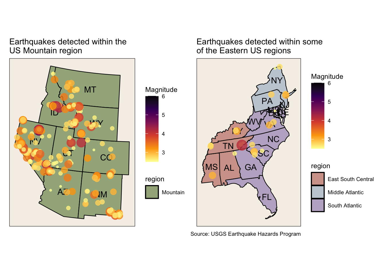
Comparing Mountain region vs Eastern regions

A comparison of quakes in these regions demonstrate just how rare quakes are on the East Coast. Further, it also emphasizes the rarity of strong tremors. Last year in Nevada there were 279 quakes of magnitude 2.5 or higher, and the largest was 4.8. The magnitude scale is logarithmic which means that each whole number increase in magnitude represents a tenfold increase in size. Recall that the earthquake in Virginia in 2011 was much larger at 5.8, and a quake of that size was would have been an incredible surprise to both East Coasters and Mountain residents. That being said, size of the earthquake alone doesn’t determine it’s intensity. The geological composition of the ground, water content, and depth of the epicenter also influence intensity.

# mountain map
mountain_map <- # USE THIS -- do mountain region vs northwest central
  plot_usmap(data = quake_count_choropleth,
             regions = "states",
             values = "region",
             labels = TRUE,
             label_color = "black",
             include = .mountain) +
  scale_fill_manual(values = c("#A3b18a")) +
  theme(legend.position = "right",
        panel.background = element_rect(color = "black", fill = "#f5f0e8")) +
  labs(title = "Earthquakes detected within the\nUS Mountain region") +
  geom_sf(data = usa_quakes |> 
            dplyr::filter(region %in% "Mountain"),
          aes(size = mag, color = mag),
          alpha = 0.8) +
  scale_color_viridis_c(
    name = "Magnitude",
    option = "inferno",
    direction = -1,
    limits = c(2.5, 6)
  ) +
  scale_size_continuous(guide = "none")

#mountain_map

# south atlantic map where Virginia is
se_mid_atlantic_map <- plot_usmap(data = quake_count_choropleth,
           regions = "states",
           values = "region",
           labels = TRUE,
           label_color = "black",
           include = c(.south_atlantic, .east_south_central, .mid_atlantic)) +
  scale_fill_manual(values = c("#d2a39a", "#C4CDD6", "#bfb1cb")) +
  theme(legend.position = "right",
        panel.background = element_rect(color = "black", fill = "#f5f0e8")) +
  labs(title = "Earthquakes detected within some\nof the Eastern US regions",
       caption = "Source: USGS Earthquake Hazards Program") +
  geom_sf(data = usa_quakes |> 
            dplyr::filter(region %in% c("South Atlantic", "East South Central", "Middle Atlantic")),
          aes(size = mag, color = mag),
          alpha = 0.8) +
  scale_color_viridis_c(
    name = "Magnitude",
    option = "inferno",
    direction = -1,
    limits = c(2.5, 6)
  ) +
  scale_size_continuous(guide = "none")+
  guides(color = guide_colorbar(order = 1))

#se_mid_atlantic_map

mountain_map + se_mid_atlantic_map

Regional Earthquake Fear and Preparedness

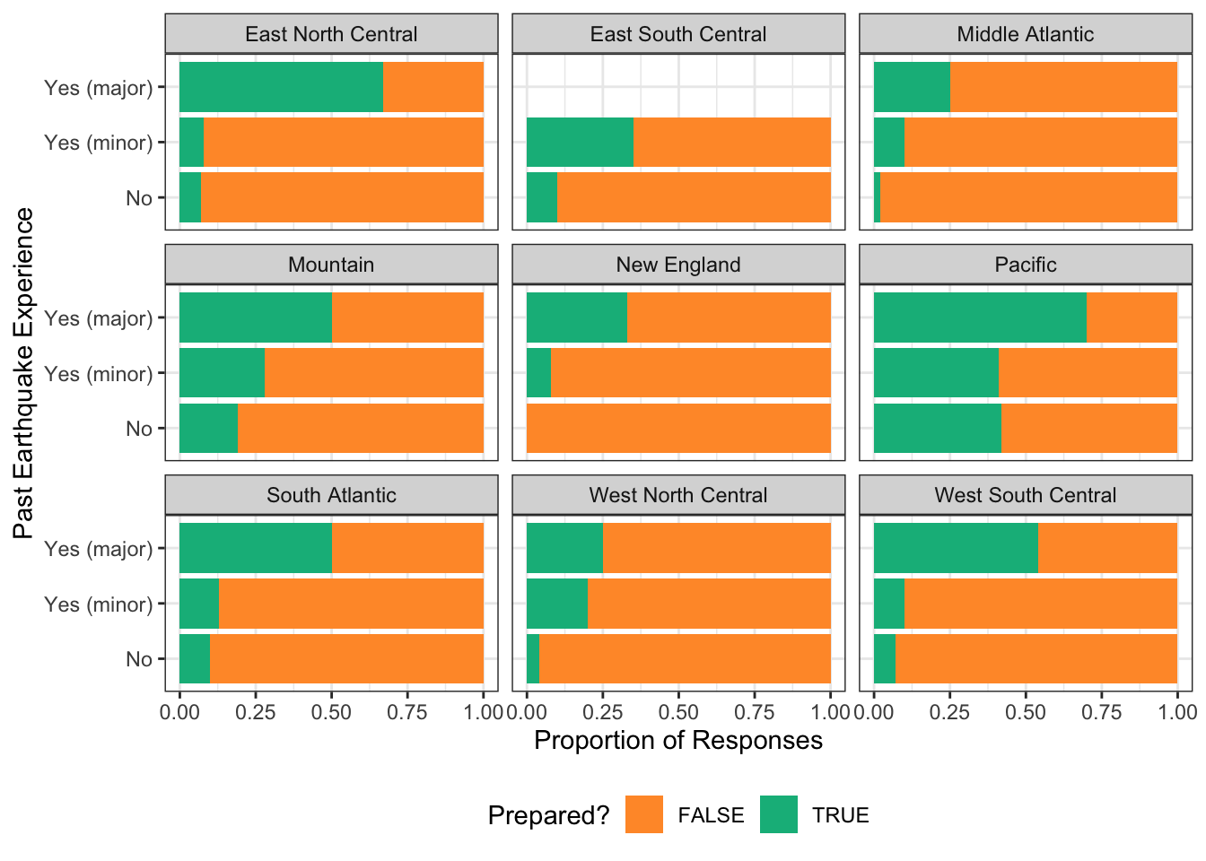
Earthquakes are extremely common in the Pacific region as these states contain very geologically active areas. As one would expect many residents in these states prepare safety precautions even when they’ve never felt even a slight tremor. Interestingly, according to a fivethirtyeight survey, even residents in regions with relatively fewer earthquakes have taken safety measures.

A note on the survey data

The survey contains responses from 1,013 people, but only 978 respondents (~97%) completed all questions. Of the 35 respondents that turned in incomplete surveys, none of them listed their US region. For analyses and data visualizations that consider region, I made the decision to exclude the incomplete data.

#sum(complete.cases(san_andreas)) # complete responses
#sum(!complete.cases(san_andreas)) # incompleted responses
#nrow(san_andreas) # total responses

#san_andreas |> dplyr::filter(is.na(region)) |> View()


san_andreas |> 
  select(region, experience, prepared) |> 
  dplyr::mutate(experience2 = case_when(experience == "No" ~ "No",
                                        experience == "Yes, one or more minor ones" ~ "Yes (minor)",
                                        experience == "Yes, one or more major ones" ~ "Yes (major)"),
                experience2 = factor(experience2, levels = c("No", "Yes (minor)", "Yes (major)"))
                ) |> 
  dplyr::group_by(region, experience2) |> 
  dplyr::count(prepared) |> 
  dplyr::mutate(proportion = round(n/sum(n),2)) |> 
  # exclude incomplete entries
  dplyr::filter(experience2 != is.na(experience2)) |>
  dplyr::filter(region != is.na(region)) |> 
  ggplot(aes(x = experience2,
             y = proportion)) +
  geom_col(aes(fill = prepared)) +
  scale_fill_manual(values = c("#ff9933", "#04b889")) +
  labs(x = "Past Earthquake Experience",
       y = "Proportion of Responses") +
  coord_flip() +
  facet_wrap(vars(region)) +
  theme_bw() +
  theme(legend.position = "bottom") +
  guides(fill = guide_legend("Prepared?"))

For example, the East South Central region (ESC) had only 10 quakes last year (the same as the East North Central (ENC) and South Atlantic (SA) regions) and none of the ESC respondents reported prior experience with a major earthquake. Curiously, a greater proportion of ESC respondents indicated that they had taken safety precautions (0.22) than either the ENC (0.09) and SA (0.14) respondents.

quake_experiences <- san_andreas |> 
  dplyr::filter(experience != is.na(experience)) |> 
  dplyr::filter(region != is.na(region)) |> 
  group_by(region, experience) |> 
  summarise(n = n()) |> 
  ungroup() |>
  dplyr::mutate(experience2 = case_when(experience == "No" ~ "No",
                                        experience == "Yes, one or more minor ones" ~ "Yes (minor)",
                                        experience == "Yes, one or more major ones" ~ "Yes (major)"),
                experience2 = factor(experience2, levels = c("No", "Yes (minor)", "Yes (major)"))
                ) |> 
  select(-experience) |> 
  rename(experience = experience2)

#head(quake_experiences)

prepped <- san_andreas |> 
  select(region, prepared) |> 
  dplyr::group_by(region) |> 
  dplyr::count(prepared) |> 
  dplyr::mutate(proportion = round(n/sum(n),2)) |> 
  dplyr::filter(region != is.na(region)) |> 
  dplyr::filter(prepared == TRUE) |> 
  select(region, proportion)

#head(prepped)

# first count number of quakes WITHIN region
# ignoring off-shore quakes
region_counts <- usa_quakes |> 
  sf::st_drop_geometry() |> 
  group_by(region) |> 
  summarise(n = n()) |> 
  dplyr::filter(!is.na(region))

# table of experience, preparedness, and number of quakes in region
quake_experiences |>
  tidyr::pivot_wider(names_from = experience,
                     values_from = n) |> 
  tidyr::replace_na(list('Yes (major)' = 0)) |> 
  mutate(Total = No + `Yes (minor)` + `Yes (major)`) |> 
  dplyr::left_join(prepped, by = "region") |> 
  rename('proportion prepped' = proportion) |> 
  left_join(region_counts, by = join_by(region)) |> 
  arrange(desc(n)) |> 
  rename("No. quakes in 2025" = n) |> 
  knitr::kable(caption = "Prior earthquake experience by US Region and proportion that have prepared safety precautions.")

Prior earthquake experience by US Region and proportion that have prepared safety precautions.

region	No	Yes (minor)	Yes (major)	Total	proportion prepped	No. quakes in 2025
Pacific	19	94	93	206	0.54	2033
Mountain	16	29	22	67	0.33	601
West South Central	46	40	13	99	0.14	525
West North Central	47	20	4	71	0.10	81
East North Central	61	76	3	140	0.09	10
East South Central	20	20	0	40	0.22	10
South Atlantic	60	85	10	155	0.14	10
Middle Atlantic	48	81	8	137	0.08	5
New England	34	26	3	63	0.05	1

It’s possible this is a sampling quirk. There could be too few ESC respondents for an accurate assessment, a some residents in Tennessee have an intense fear The Big One, or perhaps they are California transplants. But a closer look at general fears and specific fears of “The Big One” indicate that ESC respondents are not particularly worried about earthquakes.

The survey question for the prepared column was “Have you or anyone in your household taken any precautions for an earthquake (packed an earthquake survival kit, prepared an evacuation plan, etc.)?”. I suspect some ESC residents responded “yes” because they have taken precautions for other natural disasters like hurricanes, tornadoes, and floods.

# let's compare general fear of quakes in ESC, ENC, and SA
# also add Pacific as a "true" comparison

general_fears <- san_andreas |> 
  dplyr::filter(region %in% c("Pacific", "East South Central", "East North Central", "South Atlantic")
                ) |> 
  dplyr::filter(worry_general != is.na(worry_general)) |> 
  dplyr::filter(region != is.na(region)) |> 
  group_by(region, worry_general) |> 
  summarise(n = n()) |> 
  pivot_wider(values_from = n, names_from = region) |> 
  replace_na(list(`East South Central` = 0)) |> 
  rename("General Worry" = worry_general)

knitr::kable(general_fears, caption = "General fear of earthquakes by region")

General fear of earthquakes by region

General Worry	East North Central	East South Central	Pacific	South Atlantic
Not at all worried	64	16	26	57
Not so worried	49	13	60	61
Somewhat worried	16	10	83	27
Very worried	3	0	28	4
Extremely worried	8	1	9	6

big_one_fears <- san_andreas |> 
  dplyr::filter(region %in% c("Pacific", "East South Central", "East North Central", "South Atlantic")
                ) |> 
  dplyr::filter(worry_bigone != is.na(worry_bigone)) |> 
  dplyr::filter(region != is.na(region)) |> 
  group_by(region, worry_bigone) |> 
  summarise(n = n()) |> 
  pivot_wider(values_from = n, names_from = region) |> 
  replace_na(list(`East South Central` = 0)) |> 
  rename("The Big One Worry" = worry_bigone)

knitr::kable(general_fears, caption = "Fear of a massive earthquake by region.")

Fear of a massive earthquake by region.

General Worry	East North Central	East South Central	Pacific	South Atlantic
Not at all worried	64	16	26	57
Not so worried	49	13	60	61
Somewhat worried	16	10	83	27
Very worried	3	0	28	4
Extremely worried	8	1	9	6

Given the rarity of earthquakes in some regions, does it makes sense to prepare for one? What other characteristics could drive preparedness or lack thereof? The fivethirtyeight survey collected other information (such as household income, age, and sex), and you can take a closer look at the relationship between these traits and safety preparedness with this Shiny app.